Spatial Pattern Analysis Exercise
Problem: This assignment has six separate problems that need to be addressed. In exercise 8-1, a fire department needs a map that shows whether or not false alarm calls are clustering. In exercise 8-2, the fire department would like a similar map as in exercise 8-1 but they would like a fixed band width to be used. In exercise 8-3 we are interested in understanding the relationship of the clustering that we discovered in the previous exercises and the features in the map. In exercise 8-4 we are determining the density at which the patron locations of a library are clustered.
Exercises 9-1 and 9-2 are about identifying clusters. In exercise 9-1 the same fire station would like a map that shows hot spots and cold spots for the clustering of service calls with reference to the median household income for different census blocks in the area. We must then create a map that shows this information but at a fixed band width. In 9-2 We must create a map that shows high income hotspots and low income cold spots for Dallas County.
Analysis Procedures:


Strategies: For each of these exercises ArcMap was required. I used ArcMap version 10.5. The data used in each exercise was an mxd document for each separate exercise that contained all of, and only the shapefiles and table necessary for the exercise and was the accompanying data to the GIS Tutorial 2 book. Since each exercise had it own individual mxd file it was best to tackle each exercise as its own individual problem though a variation of much of these exercises could likely be done with one mxd document. The strategies implemented in this assignment are as follows:
8-1: Average Nearest Neighbor tool
8-2: High/Low Clustering (Getis-Ord General G)
8-3: Multi-Distance Spatial Cluster Analysis and Difference Calculation
8-4: Spatial Join and Spatial Autocorrelation
9-1: Cluster and Outlier Analysis (Anselin Local Moran’s I) tool
9-2: Hot-spot analysis (Getis-Ord Gi*)
Methods used in this assignment were very straightforward. For exercise 8-1 I opened the provide map document and used the nearest neighbor tool on the Incident_Feb15 layer after restricting the data so that it met the appropriate incident type and input the information on the map. For exercise 8-2 I opened the provided map, ran the High/Low Clustering (Getis-Ord General G) tool six times with varying distances until I found the highest 7 score and reported the results on the map. For exercise 8-3 I opened the provided map, ran the Multi-Distance Spatial Cluster Analysis with 9 distance bands with a confidence envelope of 99 permutations. The resulting K function graph was then added beneath the title and a graph was created. I then added a new field in the graph and calculated a difference field. I then ran the Spatial Cluster analysis again and created a graph using the difference field. The graphs were added to the map for comparison. For Exercise 8-4 I used the provided map document, performed a spatial join of the grid using Patron Locations and ran a Spatial Autocorrelation for the new grid layer.
For Exercise 9-1 I first ran the Cluster and Outlier Analysis (Local Moran’s I) tool set to the defaults to create a map. I then Used the Cluster and Outlier Analysis (Local Moran’s I) with a fixed band width to create two separate maps. For Exercise 9-2 I opened the provided map document and ran the Hot-Spot Analyisis (Geti-Ord Gi*) tool with the P053001 field with a distance 5280 and added statement about the significance of the results to the map.
Results:
Analysis of February 15 Battalion 2 calls using the Nearest neighbor index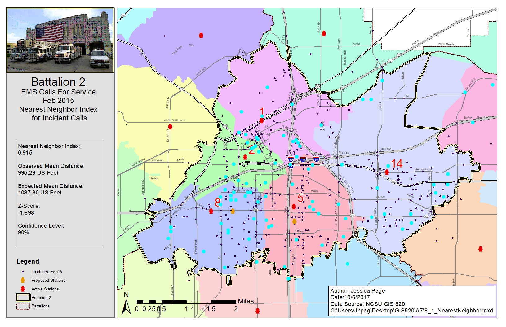
Analysis of Battalion 2 calls using the Getis-Ord General G, High Low Clustering tool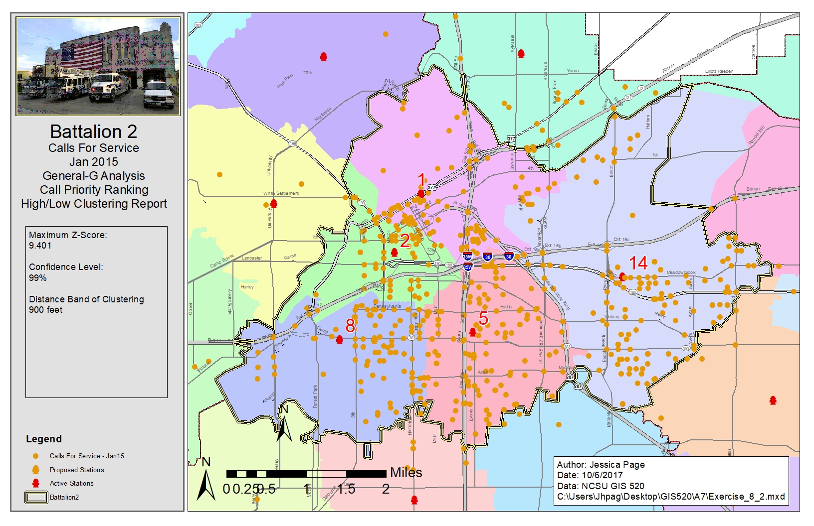
Analysis of Battalion 2 calls using the Multi-Distance Spatial Cluster Analysis and Difference Calculation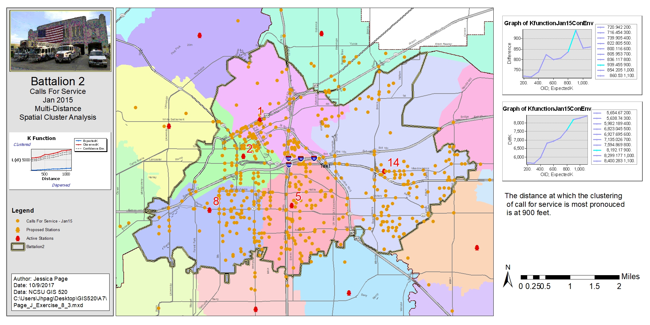
Analysis of Library Patronage using Spatial Join and Spatial Autocorrelation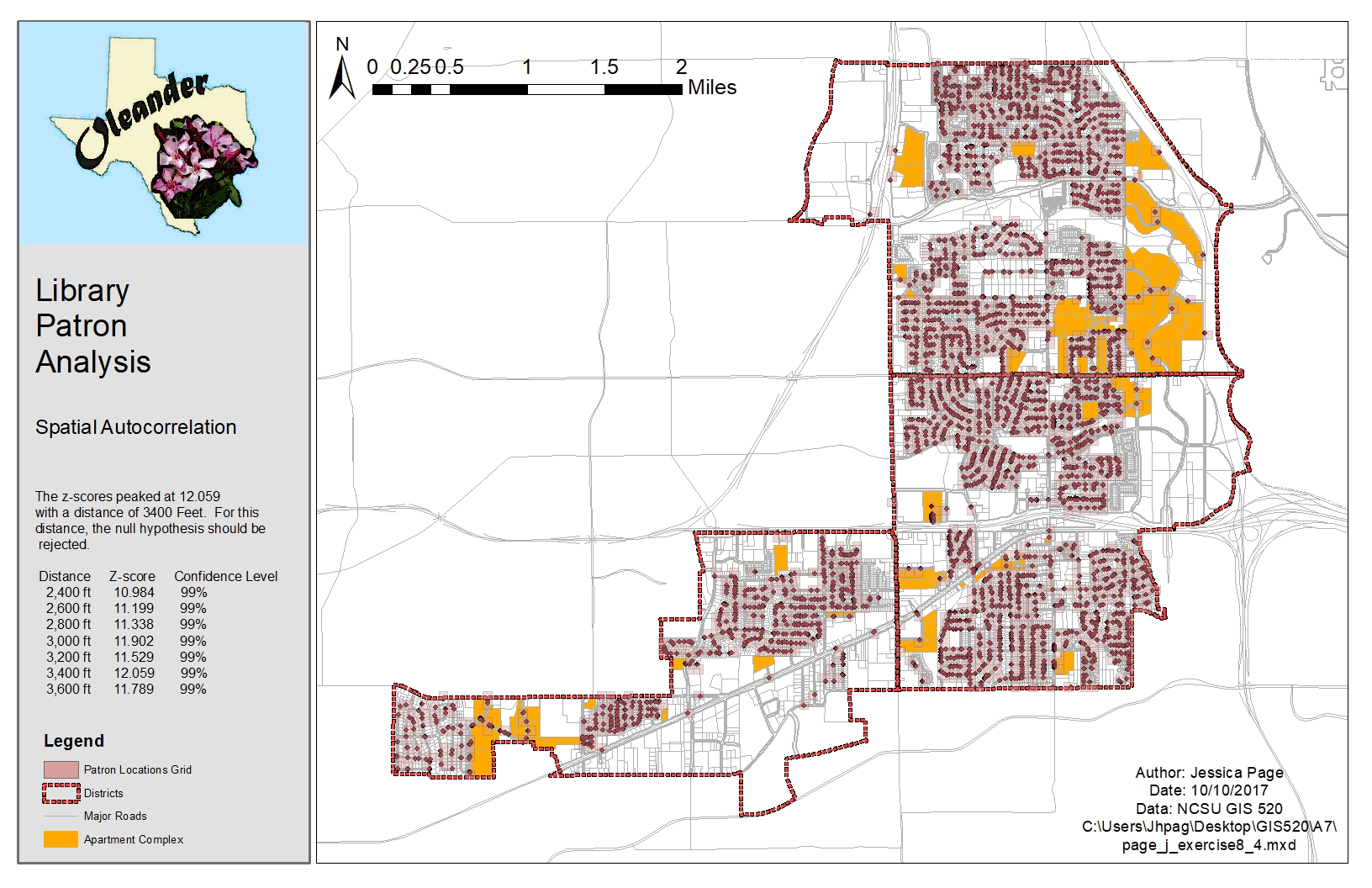
Cluster and Outlier Analysis (Anselin Local Moran’s I) tool of Battalion 2 calls without a distance band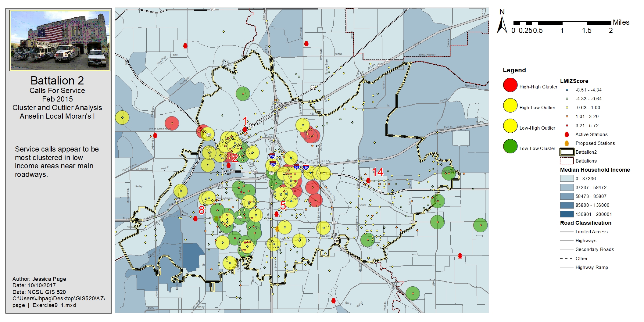
Cluster and Outlier Analysis (Anselin Local Moran’s I) tool of Battalion 2 calls with a distance band
Analysis of economic distribution in Dallas County using Hot Spot Analysis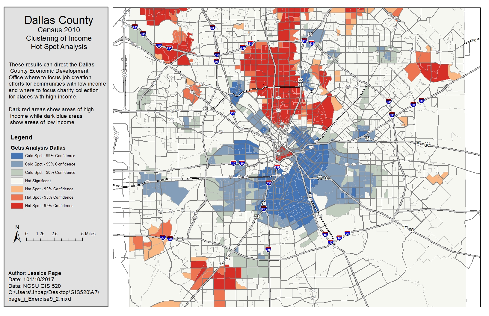
Application & Reflection: The primary theme for this assignment was using cluster analysis tools and looking for hot spots/cold spots. A good use of the tools learned in this assignment would be for something such as analyzing animal/patron land usage on a spatial scale.
Problem Description: A more specific example of this would be to look at E-birding data. As users identify birds that input that information in a database along with the location. This information would allow the analyst to determine where many of the birds are being spotted. From another perspective, it would also allow the analyst to better understand the behaviors of casual birders such as where are the birding hotspots, what might draw people to the area (such as roadways), and how can those in charge of citizen science programs reach out to more evenly distribute birding data entry.
Data Needed: Two data sources are needed for this problem. The first would be access to specific data points from E-bird which is available upon written request. The other data source would be road and feature data for the area of interest. For this example we will assume that we would like investigate potential causes for birding clusters in Wake county. This information is readily available on the county website.
Analysis Procedures: To solve this problem we would first need to run the Multi-Distance Spatial Cluster Analysis. We would then Cluster and Outlier Analysis (Anselin Local Moran’s I) tool once the appropriate distance band has been determined to look for clusters and what features/roadways they may relate to.
Additional Resources from ESRI: